Sunday, 20 August 2017
Monday, 24 July 2017
Friday, 21 July 2017
Saturday, 27 May 2017
Sunday, 21 May 2017

Saturday, 13 May 2017


Friday, 14 April 2017
Wednesday, 12 April 2017
Sunday, 9 April 2017
Thursday, 30 March 2017

Monday, 20 March 2017
Tuesday, 14 March 2017
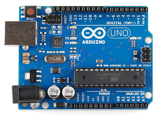
Arduino technolodgy and its development
Do you know Arduino borrowed its name from a nearby watering hole called Bar di Re Arduino where it was first developed in Italy?

15 Arduino Projects that you will Love to See
From Bluetooth Door-Lock, JPEG Camera, Heart-Pulse Alarm, Big size Wall Clock, Oscilloscope, Lie-Detector, Weather Machine, Time-Lapse Panorama Controller to even a Voting Machine.
Learn More
ARTICLES.ELECTRONICSINFOLINE.COM


Monday, 13 March 2017

Sunday, 12 March 2017
Electrical Projects
http://nevonprojects.com/engineering-projects-2/electrical-engineering-projects/http://nevonprojects.com/engineering-projects-2/electrical-engineering-projects/
Saturday, 11 March 2017
The Lorentz forces and law
The Lorentz force

The flow of an electric current down a conducting wire is ultimately due to the motion of electrically charged particles (in most cases, electrons) through the conducting medium. It seems reasonable, therefore, that the force exerted on the wire when it is placed in a magnetic field is really the resultant of the forces exerted on these moving charges. Let us suppose that this is the case. Let $A$ be the (uniform) cross-sectional area of the wire, and let $n$ be the number density of mobile charges in the conductor. Suppose that the mobile charges each have charge $q$ and velocity ${\bf v}$. We must assume that the conductor also contains stationary charges, of charge $-q$ and number density $n$ (say), so that the net charge density in the wire is zero. In most conductors, the mobile charges are electrons and the stationary charges are atomic nuclei. The magnitude of the electric current flowing through the wire is simply the number of coulombs per second which flow past a given point. In one second, a mobile charge moves a distance $v$, so all of the charges contained in a cylinder of cross-sectional area $A$ and length $v$ flow past a given point. Thus, the magnitude of the current is $q n A v$. The direction of the current is the same as the direction of motion of the charges, so the vector current is ${\bf I}' = q nA {\bf v}$. According to Eq. (229), the force per unit length acting on the wire is \begin{displaymath} {\bf F} = q n A {\bf v}\times{\bf B}. \end{displaymath} (232) However, a unit length of the wire contains $nA$ moving charges. So, assuming that each charge is subject to an equal force from the magnetic field (we have no reason to suppose otherwise), the force acting on an individual charge is \begin{displaymath} {\bf f} = q {\bf v} \times{\bf B}. \end{displaymath} (233) We can combine this with Eq. (169) to give the force acting on a charge $q$ moving with velocity ${\bf v}$ in an electric field ${\bf E}$ and a magnetic field ${\bf B}$: \begin{displaymath} {\bf f} = q {\bf E} + q {\bf v} \times{\bf B}. \end{displaymath} (234) This is called the Lorentz force law, after the Dutch physicist Hendrik Antoon Lorentz who first formulated it. The electric force on a charged particle is parallel to the local electric field. The magnetic force, however, is perpendicular to both the local magnetic field and the particle's direction of motion. No magnetic force is exerted on a stationary charged particle. The equation of motion of a free particle of charge $q$ and mass $m$ moving in electric and magnetic fields is \begin{displaymath} m\frac{d{\bf v}}{dt} = q {\bf E} + q {\bf v} \times{\bf B}, \end{displaymath} (235) according to the Lorentz force law. This equation of motion was first verified in a famous experiment carried out by the Cambridge physicist J.J. Thompson in 1897. Thompson was investigating cathode rays, a then mysterious form of radiation emitted by a heated metal element held at a large negative voltage (i.e., a cathode) with respect to another metal element (i.e., an anode) in an evacuated tube. German physicists held that cathode rays were a form of electromagnetic radiation, whilst British and French physicists suspected that they were, in reality, a stream of charged particles. Thompson was able to demonstrate that the latter view was correct. In Thompson's experiment, the cathode rays passed though a region of ``crossed'' electric and magnetic fields (still in vacuum). The fields were perpendicular to the original trajectory of the rays, and were also mutually perpendicular. Let us analyze Thompson's experiment. Suppose that the rays are originally traveling in the $x$-direction, and are subject to a uniform electric field $E$ in the $z$-direction and a uniform magnetic field $B$ in the $-y$-direction. Let us assume, as Thompson did, that cathode rays are a stream of particles of mass $m$ and charge $q$. The equation of motion of the particles in the $z$-direction is \begin{displaymath} m \frac{d^2 z}{dt^2} = q\left(E - v B\right), \end{displaymath} (236) where $v$ is the velocity of the particles in the $x$-direction. Thompson started off his experiment by only turning on the electric field in his apparatus, and measuring the deflection $d$ of the ray in the $z$-direction after it had traveled a distance $l$ through the electric field. It is clear from the equation of motion that \begin{displaymath} d = \frac{q}{m} \frac{E t^2}{2} = \frac{q}{m} \frac{E l^2}{2 v^2}, \end{displaymath} (237) where the ``time of flight'' $t$ is replaced by $l/v$.

This formula is only valid if $d\ll l$, which is assumed to be the case. Next, Thompson turned on the magnetic field in his apparatus, and adjusted it so that the cathode ray was no longer deflected. The lack of deflection implies that the net force on the particles in the $z$-direction was zero. In other words, the electric and magnetic forces balanced exactly. It follows from Eq. (236) that with a properly adjusted magnetic field strength \begin{displaymath} v = \frac{E}{B}. \end{displaymath} (238) Thus, Eqs. (237) and (238) and can be combined and rearranged to give the charge to mass ratio of the particles in terms of measured quantities: \begin{displaymath} \frac{q}{m} = \frac{2 d E}{l^2 B^2}. \end{displaymath} (239) Using this method, Thompson inferred that cathode rays were made up of negatively charged particles (the sign of the charge is obvious from the direction of the deflection in the electric field) with a charge to mass ratio of $-1.7\times 10^{11}$ C/kg. A decade later, in 1908, the American Robert Millikan performed his famous ``oil drop'' experiment, and discovered that mobile electric charges are quantized in units of $-1.6\times 10^{-19}$ C. Assuming that mobile electric charges and the particles which make up cathode rays are one and the same thing, Thompson's and Millikan's experiments imply that the mass of these particles is $9.4\times 10^{-31}$ kg. Of course, this is the mass of an electron (the modern value is $9.1\times 10^{-31}$ kg), and $-1.6\times 10^{-19}$ C is the charge of an electron. Thus, cathode rays are, in fact, streams of electrons which are emitted from a heated cathode, and then accelerated because of the large voltage difference between the cathode and anode. Consider, now, a particle of mass $m$ and charge $q$ moving in a uniform magnetic field, ${\bf B} = B \hat{\bf z}$. According, to Eq. (235), the particle's equation of motion can be written: \begin{displaymath} m \frac{d{\bf v}}{dr} = q {\bf v}\times{\bf B}. \end{displaymath} (240) This reduces to $\displaystyle \frac{dv_x}{dt}$ $\textstyle =$ $\displaystyle {\mit\Omega} v_y,$ (241) $\displaystyle \frac{dv_y}{dt}$ $\textstyle =$ $\displaystyle -{\mit\Omega} v_x,$ (242) $\displaystyle \frac{d v_z}{dt}$ $\textstyle =$ $\displaystyle 0.$ (243) Here, ${\mit\Omega} = q B/m$ is called the cyclotron frequency. The above equations can be solved to give $\displaystyle v_x$ $\textstyle =$ $\displaystyle v_\perp \cos({\mit\Omega} t),$ (244) $\displaystyle v_y$ $\textstyle =$ $\displaystyle - v_\perp \sin({\mit\Omega} t),$ (245) $\displaystyle v_z$ $\textstyle =$ $\displaystyle v_\parallel,$ (246) and $\displaystyle x$ $\textstyle =$ $\displaystyle \frac{v_\perp}{\mit\Omega} \sin({\mit\Omega} t),$ (247) $\displaystyle y$ $\textstyle =$ $\displaystyle \frac{v_\perp}{\mit\Omega} \cos({\mit\Omega} t),$ (248) $\displaystyle z$ $\textstyle =$ $\displaystyle v_\parallel t.$ (249) According to these equations, the particle trajectory is a spiral whose axis is parallel to the magnetic field. The radius of the spiral is $\rho=v_\perp/{\mit\Omega}$, where $v_\perp$ is the particle's constant speed in the plane perpendicular to the magnetic field. The particle drifts parallel to the magnetic field at a constant velocity, $v_\parallel$. Finally, the particle gyrates in the plane perpendicular to the magnetic field at the cyclotron frequency. Finally, if a particle is subject to a force ${\bf f}$ and moves a distance $\delta {\bf r}$ in a time interval $\delta t$, then the work done on the particle by the force is \begin{displaymath} \delta W = {\bf f}\cdot \delta {\bf r}. \end{displaymath} (250) The power input to the particle from the force field is \begin{displaymath} P = \lim_{\delta t\rightarrow 0} \frac{\delta W}{\delta t} = {\bf f}\cdot {\bf v}, \end{displaymath} (251) where ${\bf v}$ is the particle's velocity. It follows from the Lorentz force law, Eq. (234), that the power input to a particle moving in electric and magnetic fields is \begin{displaymath} P = q {\bf v}\cdot {\bf E}. \end{displaymath} (252) Note that a charged particle can gain (or lose) energy from an electric field, but not from a magnetic field. This is because the magnetic force is always perpendicular to the particle's direction of motion, and, therefore, does no work on the particle [see Eq. (250)]. Thus, in particle accelerators, magnetic fields are often used to guide particle motion (e.g., in a circle) but the actual acceleration is performed by electric fields.

Monday, 6 March 2017
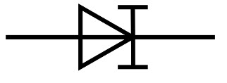
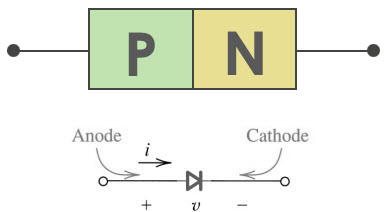
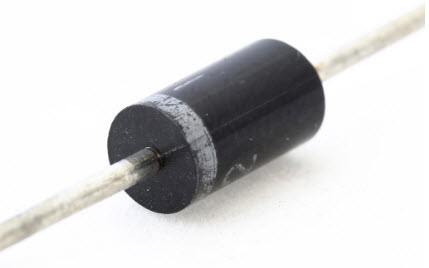
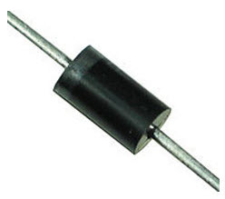
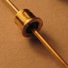
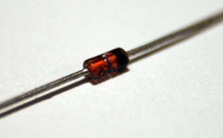
Different Types of Diodes and Their Uses
A diode is a two-terminal electrical device, that allows the transfer of current in only one direction.The diode is also known for their unidirectional current property, where the electric current is permitted to flow in one direction. Basically, a diode is used for rectifying waveforms, within radio detectors or within power supplies.They can also be used in various electrical and electronic circuits where ‘one-way’ result of the diode is required. Most of the diodes are made from semiconductors like Si (silicon), but sometimes, Ge (germanium) is also used.It is sometimes beneficial to summarize the different types of diodes are existing. Some of the types may overlap, but the various definitions may benefit to narrow the field down and offer an overview of the different diode types.
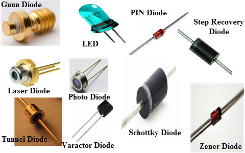
Different Types of Diodes
There are several types of diodes are available for use in electronics design, namely; a Backward diode, BARITT diode, Gunn Diode, Laser diode, Light emitting diodes, Photodiode, PIN diode, PN Junction, Schottky diodes, Step recovery diode, Tunnel diode, Varactor diode and a Zener diode.
Backward Diode
This type of diode is also called the back diode, and it is not widely used. The backward diode is a PN-junction diode that is similar to the tunnel diode in its process. It finds a few special applications where its specific properties can be used.
BARITT Diode
The short term of this diode Barrier Injection Transit Time diode is BARITT diode. It is applicable in microwave applications and allows many comparisons to the more widely used IMPATT diode. Please refer the below link for BARRITT Diode
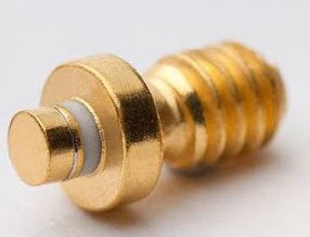
Gunn Diode
Gunn diode is a PN junction diode, this sort of diode is a semiconductor device that has two terminals. Generally, it is used for producing microwave signals. Please refer the below link for Gunn Diode Working, Characteristics, and its Applications
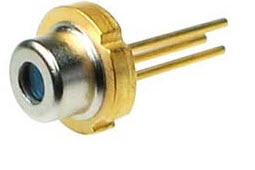
Laser Diode
The laser diode is not the similar as the ordinary LED (light emitting diode) because it generates coherent light. These diodes are extensively used in many applications like DVDs, CD drives and laser light pointers for PPTs. Although these diodes are inexpensive than other types of laser generator, they are much more expensive than LEDs. They also have a partial life.Please refer the below link for: for: How to Make a Laser Pointer
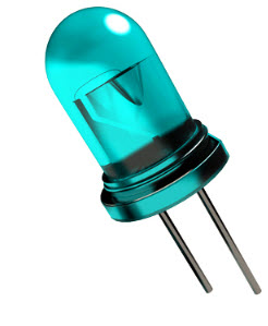
Light Emitting Diode
The term LED stands for light emitting diode, is one of the most standard types of the diode. When the diode is connected in forwarding bias, then the current flows through the junction and generates the light. There are also many new LED developments are changing they are LEDs and OLEDs.Please refer the below link for: LED light sources
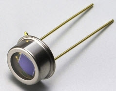
Photodiode
The photodiode is used to detect light. It is found that when light strikes a PN-junction it can create electrons and holes. Typically, photodiodes operate under reverse bias condition where even a small amount of flow of current resulting from the light can be simply noticed. These diodes can also be used to produce electricity.Please refer the below link for Photodiode Working Principle, and Its Characteristics
PIN Diode
This type of diode is characterized by its construction. It has the standard P-type & N-type regions, but the area between the two regions namely intrinsic semiconductor has no doping. The region of the intrinsic semiconductor has the effect of increasing the area of the depletion region which can be beneficial for switching applications.Please refer the below link for PIN Diode Basics, Working, and Its Applications.
PN Junction Diode
The standard PN junction may be thought of as the normal or standard type of diode in use today. These diodes can come as small signal types for use in RF (radio frequency), or other low current applications which may be called as signal diodes. Other types may be planned for high voltage and high current applications and are normally named rectifier diodes.Please refer the below link for PN Junction Diode Theory and VI Characteristics
Schottky Diode
The Schottky diode has a lower forward voltage drop than ordinary Si PN-junction diodes. At low currents, the voltage drop may be between 0.15 & 0.4 volts as opposed to 0.6 volts for a Si diode. To attain this performance they are designed in a different way to compare with normal diodes having a metal to semiconductor contact. These diodes are extensively used in rectifier application, clamping diodes, and also in RF applications.Please refer the below link for Schottky Diode Working and Applications
Step Recovery Diode
A step recovery diode is a type of microwave diode used to generate pulses at very HF (high frequencies). These diodes depend on the diode which has a very fast turn-off characteristic for their operation.
Tunnel Diode
The tunnel diode is used for microwave applications where its performance surpassed that of other devices of the day.Please refer the below link for Tunnel Diode Circuit with Operation and Its Applications.
Varactor Diode or Varicap Diode
A varactor diode is one sort of semiconductor microwave solid-state device and it is used in where the variable capacitance is chosen which can be accomplished by controlling voltage. These diodes are also called as variceal diodes. Even though the o/p of the variable capacitance can be exhibited by the normal PN-junction diodes.But, this diode is chosen for giving the preferred capacitance changes as they are different types of diodes. These diodes are precisely designed and enhanced such that they allow a high range of changes in capacitance. Please refer the below link for Varactor Diode Working and Its Applications .
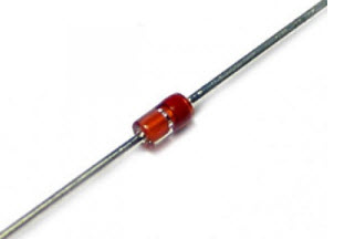
Zener Diode
The Zener diode is used to provide a stable reference voltage. As a result, it is used in vast amounts. It works under reverse bias condition and found that when a particular voltage is reached it breaks down. If the flow of current is limited by a resistor, it activates a stable voltage to be generated. This type of diode is widely used to offer a reference voltage in power supplies. Please refer the below link for Zener Diode Circuit Working and Its Applications.
Thus, this is all about different types of diodes and its uses.We hope that you have got a better understanding of this concept or to implement electrical projects please give your valuable suggestions by commenting in the comment section below. Here is a question for you, What is the function of a diode?
Subscribe to:
Posts (Atom)
